Author: pogcha
Protected: DPG-2016
Adding links to title or year in Latex Bibliography
I tried to achieve that latex adds links (dois or urls) to the references without showing the ugly url/doi in the reference. I believe nobody has ever benifited by reading those url/dois in a print version by typing the text into the browser. The revtex format of APS does something like that by a sophisticated style file for bibtex (.bst). However, I did not succeed in replicating this behavior with my own bst file. My workaround is to alter the .bib file direclty to interchange every title/year entry
year = { 2006 }
by a
year = { \href{ \href{http://dx.doi.org/... }{ 2006 } }
I did this with a python script and it works perfectly fine with the caveat of having one extra script and step in generating a document from tex source.
Simply run the python script by
python makeDoiLink.py
and you will be promted for the file name and if you want to add the link to title or year. The output will be a new .bib file called oldfileDOI.bib.
Please download and feel free to use and alter the script
makeDoiLink.py
Zotero: Fix Latex math commands in Bibtex export
Locate your Zotero data directory and edit translators/BibTeX.js
1) Change
var alwaysMap = {
  "|":"{\\textbar}",
  "<":"{\\textless}",
  ">":"{\\textgreater}",
  "~":"{\\textasciitilde}",
  "^":"{\\textasciicircum}"
  "\\":"{\\textbackslash}",
  "{" : "\\{\\vphantom{\\}}",
  "}" : "\\vphantom{\\{}\\}"
}
to
var alwaysMap = {
  "|":"{\\textbar}",
  "<":"{\\textless}",
  ">":"{\\textgreater}",
  "~":"{\\textasciitilde}",
  "^":"^"
  "\\":"\\",
  "{" : "{",
  "}" : "}"
}
2) Change
function escapeSpecialCharacters(str) {
  var newStr = str.replace(/[|\<\>\~\^\\\{\}]/g, function(c) { return alwaysMap[c] })
    .replace(/([\#\$\%\&\_])/g, "\\$1");
to
function escapeSpecialCharacters(str) {
  var newStr = str.replace(/[|\<\>\~\^\\\{\}]/g, function(c) { return alwaysMap[c] })
    .replace(/([\#\%\&])/g, "\\$1");
This should do the trick. The instructions are tested for Zotero 4.0.28.1
This based on http://www.ohadsoft.com/2012/06/zotero-exporting-unicode-and-latex-constructs-to-bibtex/ which seems to be for an older version of Zotero.
This is somewhat related: When exporting items by right click… export as… zotero displays the option to use abbreviated journal names. This is not the case for exporting by using quick copy. This can be fixed by again editing the translator file. To do so, simply change the option “useJournalAbbreviation” of “displayOptions” to “true”. You find this entry in the header of the file.
Script to convert between natural units and SI units
The SI unit system and the natural unit system are equivalent ways of describing physical quantities. SI has the basis (meter, second, kilogram and Ampere). The natural system has the basis (speed of light, , electron volt, and
).
This python script makes it easy and transparent to convert quantities between these systems. It is a simple command line tool, which is invoked with the value you want to convert, its unit system and the powers of its units. An easy example would be to check, if the speed of light, 2.998 108 m/s, is ‘one’ in natural units. The power of meter is 1, the power of seconds is -1. The powers of the remaining kg and A are both 0. Running the code then looks like this
convert_SI_Natural.py --unit=si -- 2.998e8 1 -1 0 0
 converted
   2.998000000e+08 m s^-1
 = 1.000025157e+00 c
Looks good! Now lets check the opposite direction. The power of c is 1. The powers of the remaining units (, eV and
) are zero.
convert_SI_Natural.py --unit=nat -- 1.0 1 0 0 0
 converted
   1.000000000e+00 c
 = 2.997924580e+08 m s^-1
This is the value by NIST definition. All the details for using the script can be found by invoking the script with
convert_SI_Natural.py --help
Download and have fun.
convert_SI_Natural.py
Doping dependent Fermi surface of graphene
This animation shows the Fermi surface of graphene for different dopings. The left panel shows the Brioullin zone in the k-space and the Fermi surfaces. The left panel shows the density of states and the right one the dispersion of graphene. The different doping levels are depicted as a line at the Fermi energy moving up in the dispersion and density of states.
One can nicely see the disappearence of the Fermi surface around the K points (corners of the Brillouin zone) for neutral Graphene (zero Fermi energy). In the parabolic regions of the dispersion, near the Gamma point for very low and very high dopings, the Fermi surface is a circle in very good approximation. In between the circular Fermi surface and the dot like Fermi surface, it has a triangular shape around the K points. Another interesting point to note is the fact that the Fermi surface changes its center from the Gamma point to the K point right at the van Hove singularities at 1eV.
The dispersion is calculated by the nearest neighbor tight-binding approximation, c.f. Rev. Mod. Phys. 81, 109
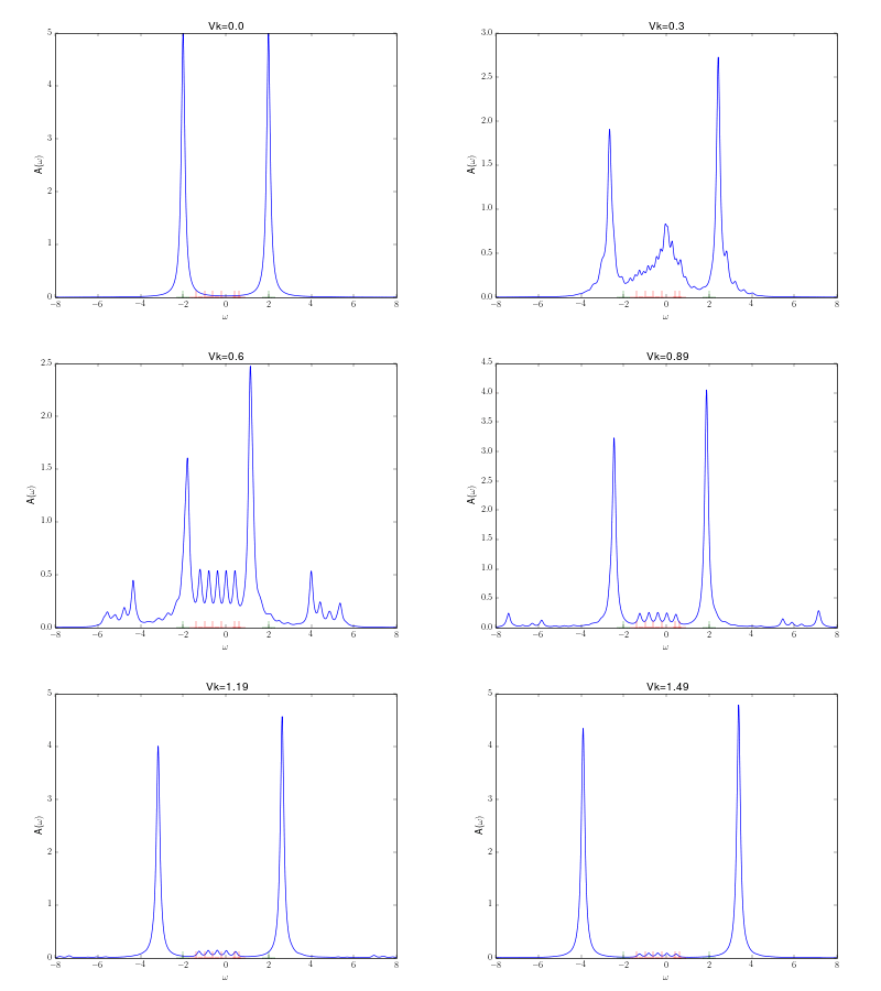
Evolution of the spectral function for the AIM
This animation shows the evolution for a simple Anderson impurity model (AIM) for rising hybridization strength from the atomic limit to a strongly coupled system.
The Hamiltonian reads with bath energies
marked in red in the graph (implicit spin summation).
The excitation energies of the atomic limit at and
are marked in green. A nice evolution from the atomic spectrum at small hybridizations with lower and upper Hubbard peaks over some kind of a Kondo resonance at the Fermi energy for intermediate hybridizations (
) to a fully coupled system with two peaks corresponding to the bonding and anti bonding orbital, one wandering down and one up in energy with increasing hybridization.

